K-Means Example: Iris
Clustering Iris dataset
1- K-Means Cluster Model
‘http://altanalyze.blogspot.com/2012/06/hierarchical-clustering-heatmaps-in.html
a) Python Libraries for KMeans
We can use KMeans from Scikit-Learn’s cluster module to build a KMeans model for clustering.
Let’s import the needed libraries to use first.
from sklearn.cluster import KMeans
import seaborn as sns
import matplotlib.pyplot as plt
from sklearn.datasets import load_iris
import numpy as np
import pandas as pd
b) Built-in Iris Dataset
We can then build an array using the feature values in the Iris dataset. Please note that we’re going to need labels, classes or test partitions etc. as we’re not going to predict classes or target.
For clustering all we need is data without labels and clustering algorithm will do the rest. So let’s load the Iris dataset and create an array named X.
data = load_iris()
Xall = data.data[:]
X_data = data.data
print(X_data[:3])
[[5.1 3.5 1.4 0.2]
[4.9 3. 1.4 0.2]
[4.7 3.2 1.3 0.2]]
Great we only have the raw feature values assigned to X. And actually I’d like to use only two columns for demonstration purposes. This way we can plot clusters on a 2-D scatter chart.
X = X_data[:,0:2]
print(X[:3])
Perfect now, we are ready for clustering and visualization.
[[5.1 3.5]
[4.9 3. ]
[4.7 3.2]]
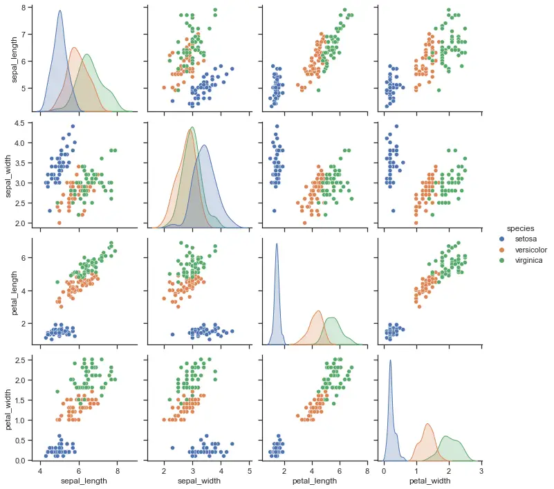
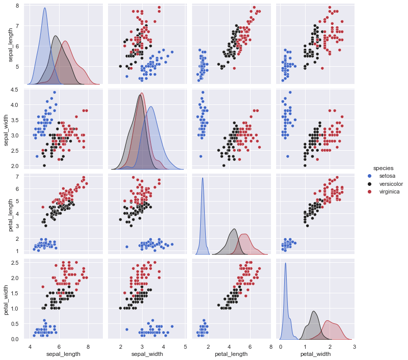
For clarification, we extracted only values sepal_length and sepal_width features from Iris dataset here. If you don’t remember Iris dataset you can check out this nice graph created with seaborn library.
It’s also nice to see because target classes from the original dataset are color mapped. So we can compare how clustering will work later.
import seaborn as sns
sns.set_theme(style="darkgrid")

df = sns.load_dataset("iris")
sns.pairplot(df, hue="species", palette="icefire")
c) Creating KMeans Cluster Model
We can create the KMeans Cluster Model by using KMeans class that we’ve already imported from sklearn.cluster library.
At this stage we can also consider some defining K-Means parameters like init, n_clusters or n_init. Please refer to this tutorial for more detail about K-Means parameters and how to optimize them:
Here we are establishing a KMeans model with default values. init defines the method for initiating K-Means centroids. k-means++ is just the default parameter and it will select initial centroids in a way that convergence for clustering will be sped up. You can also select a random centroid initiation process by assigning init to “random”.
n_clusters is the amount of clusters that will be made and we are assigning it to 5 here just for demonstration. Finally n_init is the amount of initiations that will be made with centroid seed so that the best runs can be picked. n_init is 10 by default, we’re keeping it as is for this example.
k = 5
KM = KMeans(init = "k-means++", n_clusters = k, n_init = 10)
K-Means doesn’t have training phase so we can’t talk about time complexity there but it does have a time complexity for clustering phase.
Depending on the iteration amount, cluster amount and dimensional size of data (both sample size and columns in the array) K-Means time complexity will often fall somewhere between Linear Complexity and Quadratic Complexity. You can see a more detailed explanation here:
Fitting KMeans Model
2- Creating Clusters and Cluster Centers
KM.fit(X)
After we’ve created a suitable KMeans Model, fitting it is as easy as calling the data on the model using fit method in Python. Very simple but crucial step in the process overall.
Now we have centroids and clusters. Let’s check them out.
a) Printing Cluster Labels
labels = KM.labels_
print(labels)
[2 4 4 4 2 2 4 2 4 4 2 4 4 4 2 2 2 2 2 2 2 2 2 2 4 4 2 2 2 4 4 2 2 2 4 4 2
2 4 2 2 4 4 2 2 4 2 4 2 4 3 3 3 1 3 1 3 4 3 4 4 1 1 1 1 3 1 1 1 1 1 1 1 1
3 3 3 3 1 1 1 1 1 1 1 3 3 1 1 1 1 1 1 4 1 1 1 1 4 1 3 1 0 3 3 0 4 0 3 0 3
3 3 1 1 3 3 0 0 1 3 1 0 1 3 0 1 1 3 0 0 0 3 3 1 0 3 3 1 3 3 3 1 3 3 3 1 3
3 1]
It makes sense. We have labels for each sample ranging from 0 to 4 so 5 clusters total.
b) Printing Cluster Centers
centro = KM.cluster_centers_
print(centro)
[[7.4750000 3.12500000 ]
[5.85777778 2.71333333]
[5.22068966 3.66551724]
[6.56216216 3.05945946]
[4.77777778 2.94444444]]
And, we have 5 centroids with 2 coordinations. 2 coordinations because previously we have chosen only 2 columns of Iris data so we can plot clusters on 2-D.
Plotting Individual Trees in a Random Forest
3- K-Means Cluster Visualization
Visualizations can help us further understand how K-Means performed and how clusters appear.
k = 5
KM = KMeans(n_clusters = k)
KM.fit(X)
labels = KM.labels_
centro = KM.cluster_centers_
fig, ax = plt.subplots(figsize = (8,5), dpi=800)
colors = plt.cm.prism(np.linspace(0, 1, k))
for i, col in zip(range(k), colors):
centroid = centro[i]
ax.plot(centroid[0], centroid[1], 'o', markeredgecolor='k', markersize=5, markerfacecolor=col)
ax.plot(X[labels==i, 0], X[labels==i, 1], 'wo', markerfacecolor=col, marker='.')
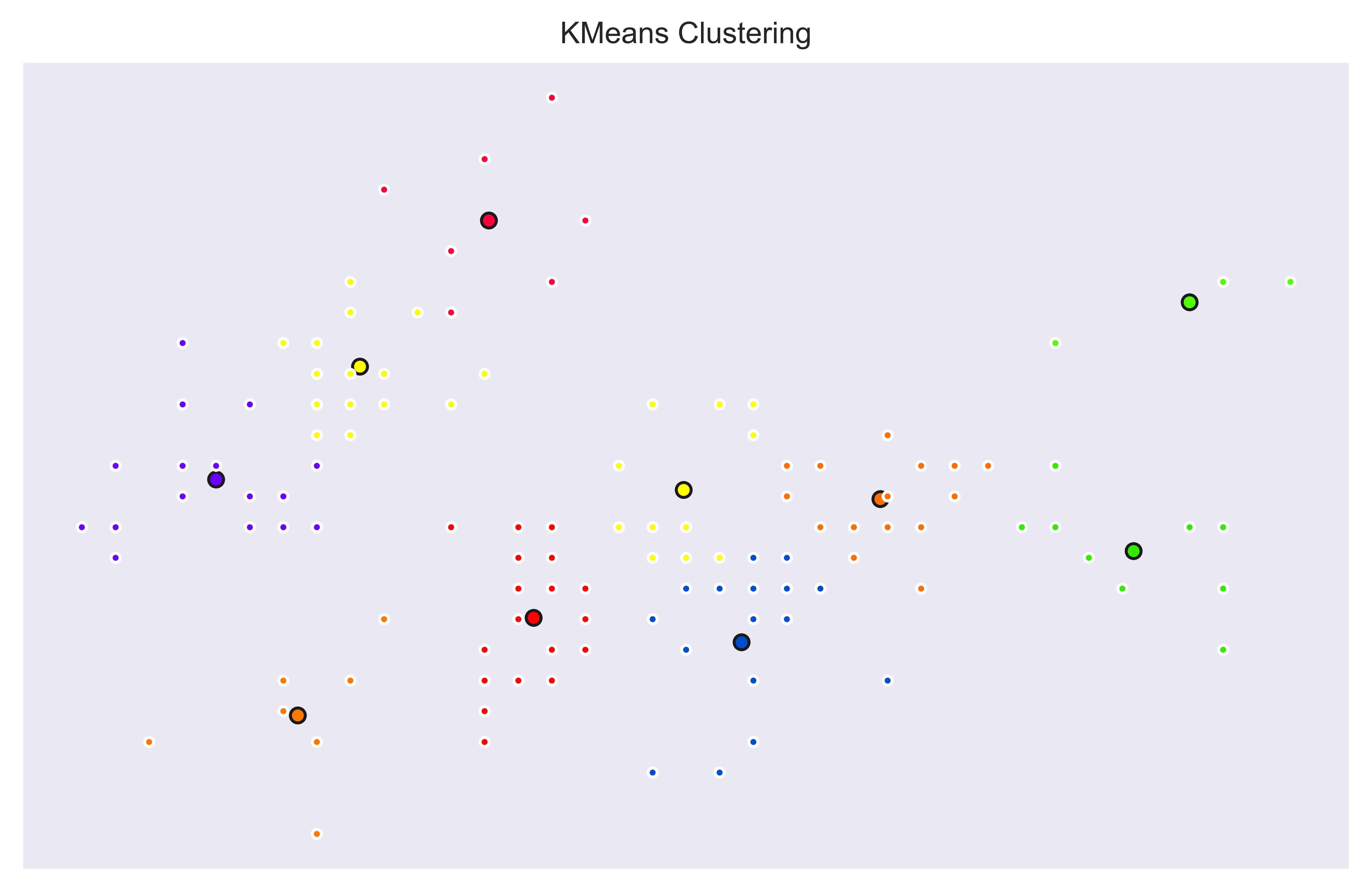
ax.set_title('KMeans Clustering', size=10); ax.set_xticks(()); ax.set_yticks(())
plt.show()
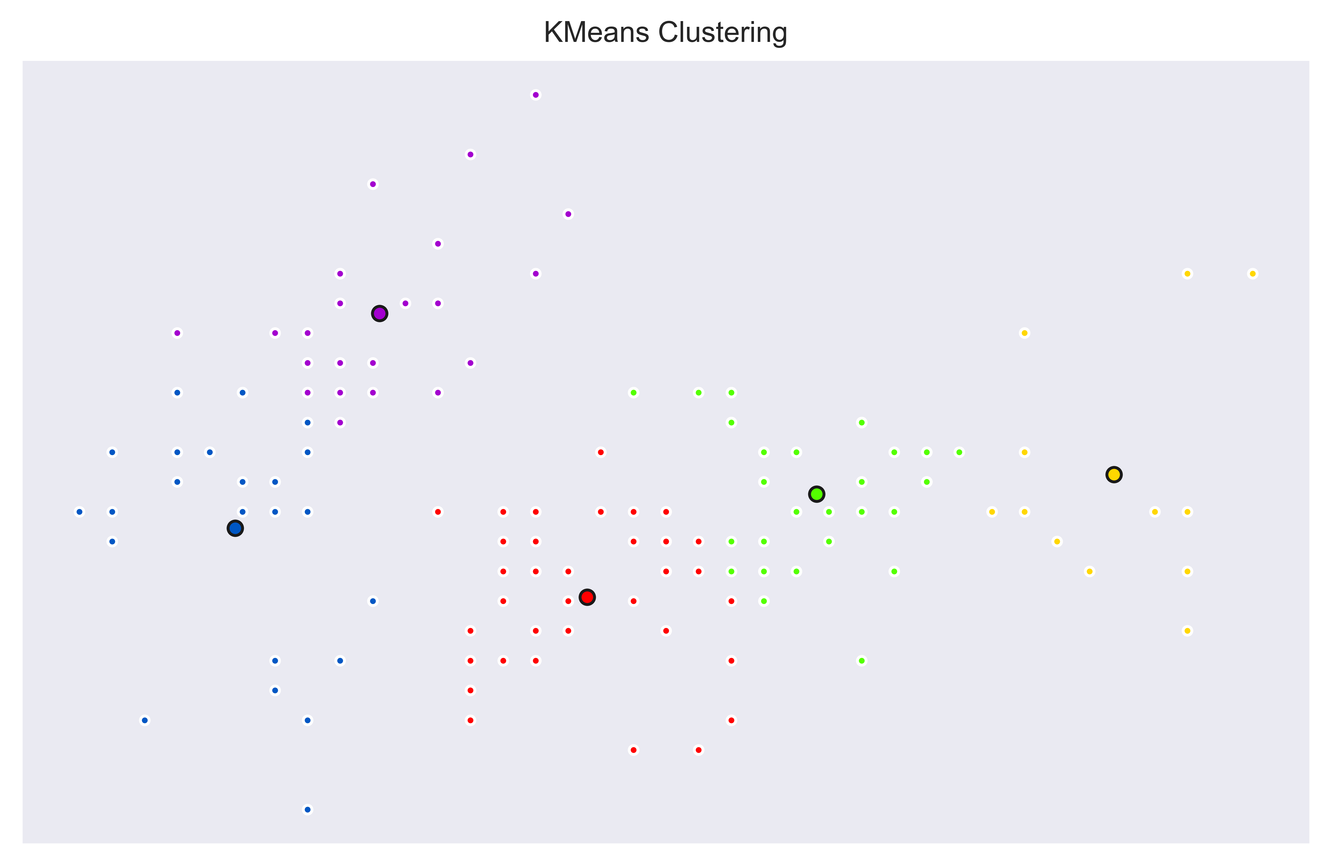
We can see 5 different clusters based on first and second columns of Iris Dataset. Interestingly, on the top left we can see that Setosa class is separated as two clusters (Blue and Purple). This is a great way to see potential sub categories and it shows us not all Setosa Iris are the same.
This type of hybrid machine learning between supervised and unsupervised methods can be very helpful to gain further insight. Similarly, we can see on the right side some members of Virginica class are also showing different clusters which also makes sense since there seems to be some members with outlier like values (Yellow dots on the very right and also top-right).
We can easily create clusters by changing the k value based on the Python code above and visualization will automatically adapt since it references k value in the plot creation also.
Let’s create 3 clusters. Here is a k=3 version with KMeans model:
And a k=10 version with KMeans model to create 10 clusters.
Plotting Individual Trees in a Random Forest
4- Clustering Using All Data
We have made some nice and simple demonstrations. Let’s work on 3 clusters now and see how clusters would occur if we’ve used all the data we have. We will fit KMeans model with 4 columns and then visualize the resulting clusters on 2 axes (using 2 input columns) and 3 axes (using 3 input columns).
Let’s create an X not only with first two columns but all columns:
X = X_data[:]
We have made some nice and simple demonstrations. Let’s work on 3 clusters now and see how clusters would occur if we’ve used all the data we have. We will fit KMeans model with 4 columns and then visualize the resulting clusters on 2 axes (using 2 input columns) and 3 axes (using 3 input columns).
Let’s create an X not only with first two columns but all columns:
k = 3
KM = KMeans(n_clusters = k)
KM.fit(X)

labels = KM.labels_
centro = KM.cluster_centers_

fig, ax = plt.subplots(figsize = (8,5), dpi=800)
colors = plt.cm.prism(np.linspace(0, 1, k))

for i, col in zip(range(k), colors):
    centroid = centro[i]
    ax.plot(centroid[0], centroid[1], 'o', markeredgecolor='k', markersize=5, markerfacecolor=col)
    ax.plot(X[labels==i, 0], X[labels==i, 1], 'wo', markerfacecolor=col, marker='.')

ax.set_title('KMeans Clustering', size=10); ax.set_xticks(()); ax.set_yticks(())
plt.show()
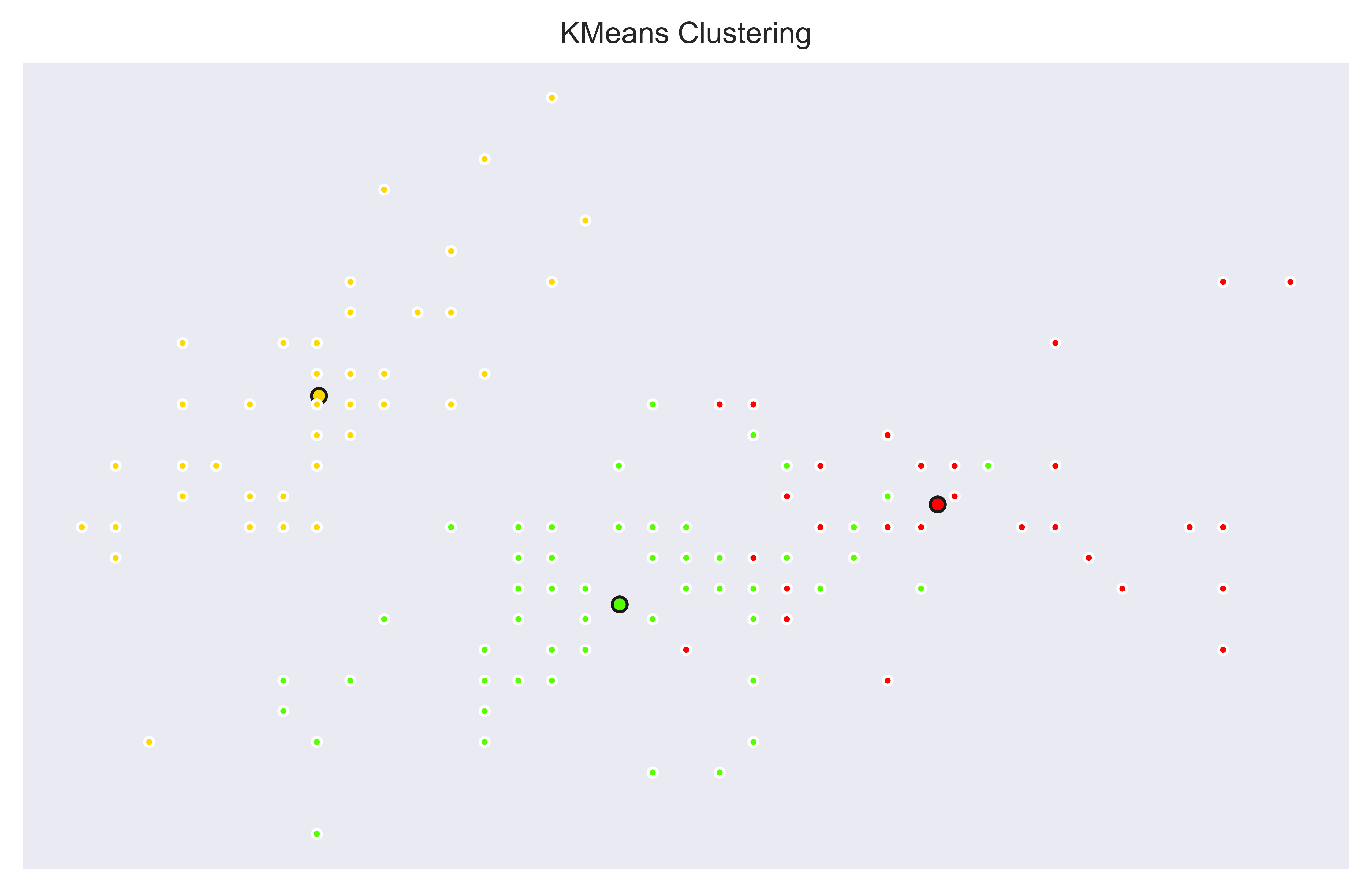
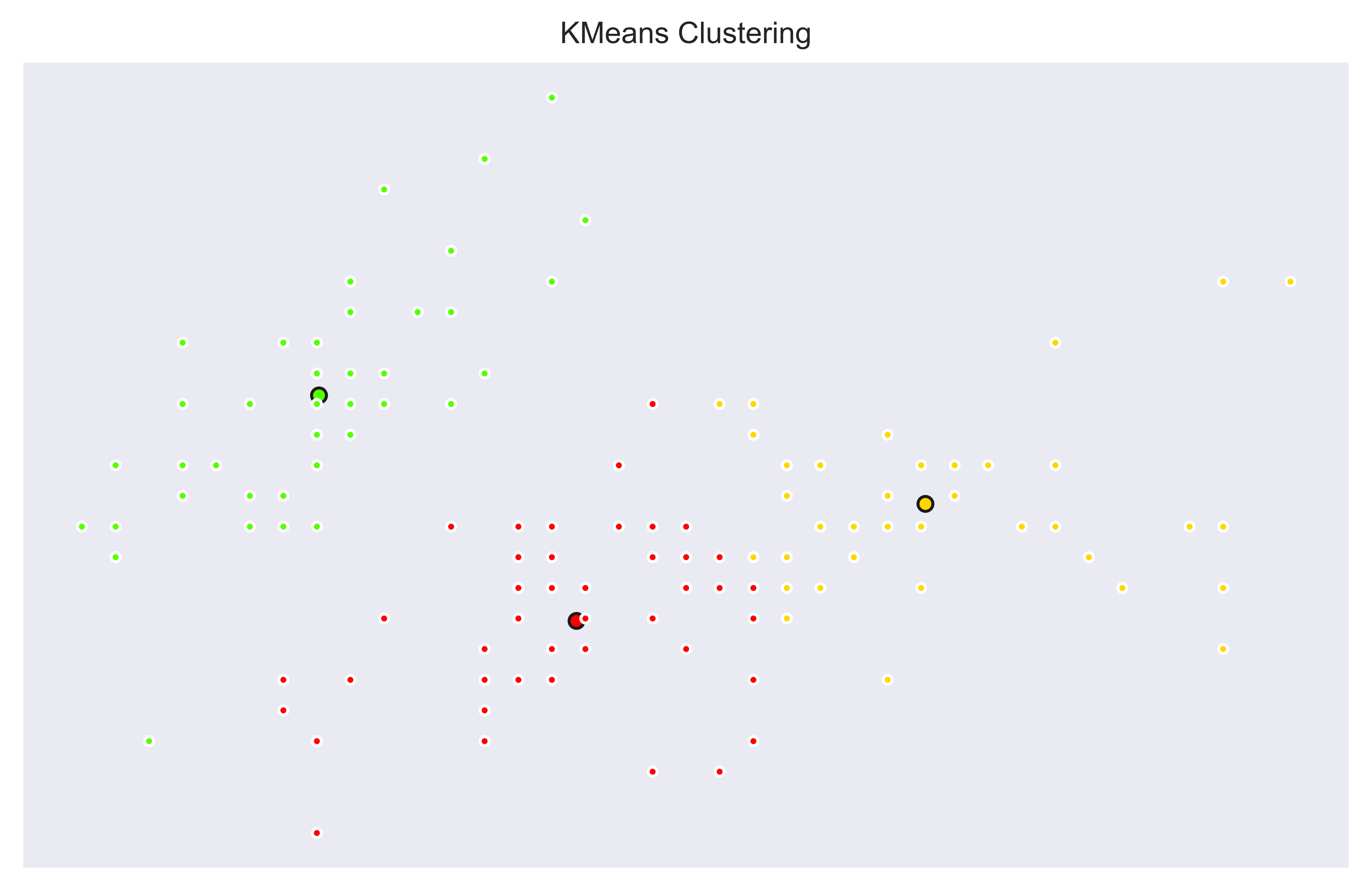
This time we can see that clusters aren’t looking like separations are as clear as before. There are some overlapping labels. This is because we are properly labeling samples based on multiple features which we don’t see all of them here. Yellow cluster is still clearly separated meaning it is separable based on only first two columns.
We can also jump to 3-D plotting features and see if there is more insight. We can visualize K-Means clustering on 3-D axes using Axes3D from mpl_toolkits,mplot3d library.
from mpl_toolkits.mplot3d import Axes3D
fig, ax = plt.subplots(figsize = (8,5), dpi=800)
plt.clf()

ax = Axes3D(fig, azim=-45)
ax.scatter(X[:, 1], X[:, 0], X[:, 2], c= labels.astype(np.float), cmap=plt.cm.prism)
ax.set_xlabel('X2'); ax.set_ylabel('X1'); ax.set_zlabel('X3')
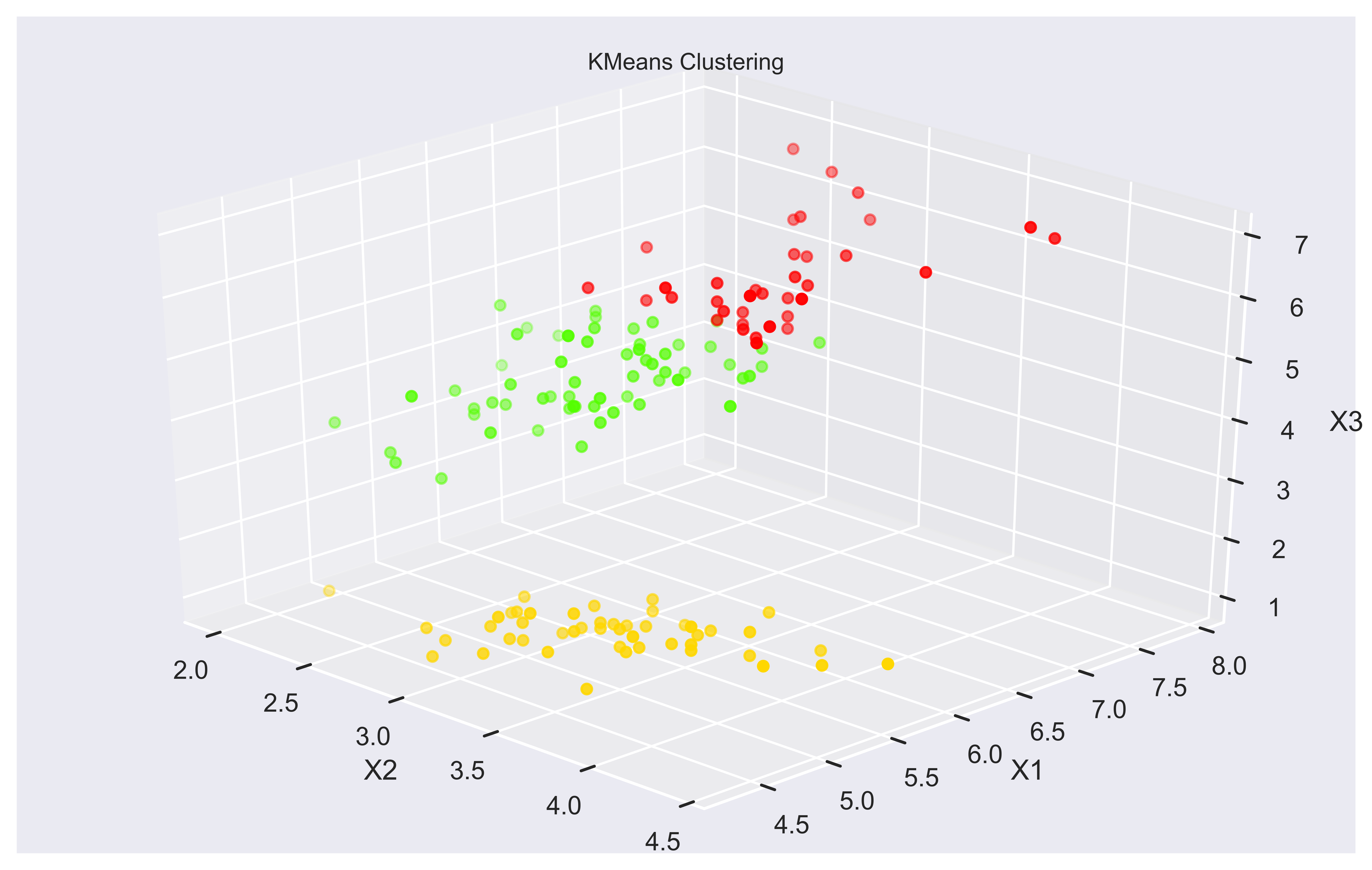
Here we can see how clusters are separated not only based on X1 and X2 but also X3 and X4 (not visible here). It makes more sense and is more intuitive.
You can play further with 3-D plot by changing azim and eval parameters. azim defines the horizontal tilt while elev can be used for adjusting the vertical tilt of the 3-D plot. azim is -60 degrees by default while elev is 30 degrees.
Also, we are using a built-in color map called prism from matplotlib library. You can see other cool color maps here.
Summary
In this part of our K-Means Tutorial Series we have implemented a K-Means Model on famous Iris dataset using KMeans class from sklearn.cluster module.
We’ve also taken advantage of visualization techniques to analyze and understand Iris dataset as well as clusters we have created using K-Means. We learned how to use specific concepts from Scikit-Learn and Matplotlib libraries of Python programming language. We have used some of the attributes of KMeans model after clustering with it to get the cluster center values and cluster label values. These attributes were:
- cluster_centers_ : for cluster centers
- labels_ : for label values
Furthermore, we’ve discussed some of the intricacies of choosing cluster centroids. And finally we have created a 3D plot to visualize cluster positions based on three different inputs.
You can apply the skills you have gained from this K-Means tutorial to your own projects to create a Machine Learning portfolio with visualizations.
You can also use K-Means clustering skills in creating innovative solutions or job searching process and recruitment as clustering is a very valuable technology that can improve many businesses processes or to gain further insight.
You can see our other Machine Learning Tutorials to continue improving your Machine Learning skillset and Machine Learning knowledge.