Support Vector Machine Example: Iris

Predicting with built-in Iris dataset

1- Support Vector Machine Classifier Model (SVC): Training & Prediction

Python and Scikit-Learn are packed with useful libraries and modules that can be used in Machine Learning projects.

We can use SVC from Scikit-Learn to create a Support Vector Classifier model for a classification project.
We can also use train_test_split to split the data to train and test partitions.
We can then use load_iris to have a dataset to work with.

Let’s import the libraries we’re going to use first.

from sklearn.svm import SVC
from sklearn.model_selection import train_test_split
from sklearn.datasets import load_iris

a) Working with built-in dataset: Iris

We’ll continue working with the iris dataset. It can be loaded using Scikit-Learn library’s load_iris module.

data = load_iris()
X = data.data
y = data.target

Now we can create a train test split and start training the SVC model.

b) Creating Train Test Split via train_test_split

This part is same for most machine learning tasks. We need to create X_train, X_test, y_train and y_test parts from the dataset.

X_train, X_test, y_train, y_test = train_test_split(X, y, test_size=0.2)

Now all the data we need is properly divided between and ready to use for training, predicting and model evaluation.

c) Creating the Model: Support Vector Machine Classifier

We can create the Random Forest model which we will implement. We can do this by using RandomForestClassifier we’ve already imported.

This is also a good stage for defining some of the parameters of the Random Forest model. Some of the most commonly adjusted parameters are: n_estimators (for tree amount), n_jobs (for parallel computing), max_depth (for tree depth) and max_features (limiting feature size). You can see more about Random Forest parameters and how to optimize them here:

Let’s create a plain vanilla random forest model with all the default settings:

SVM = SVC(kernel="rbf")

You could also create a Random Forest model with a few parameters defined specifically as following:

SVM = SVC(kernel="poly", C=100, gamma=0.0001)

You can see a more detailed tutorial about how to tune Support Vector Machines by optimizing hyperparameters through the link below:

Tuning Support Vector Machines

2- Training SVC

We have the model, we have the training data now we can start training the model.

SVM.fit(X_train, y_train)

Depending on the dataset runtime speed can change for this process. To have a clear idea about how much time it takes to train Random Forest algorithm and Random Forest complexity for scaling you can see this article:

Support Vector Machine Complexity

3- Making Predictions with SVC

After training the model it will be ready for use. Here we are making a prediction using the test partition of data without target values.

We can then compare model’s output (yhat) with target values that we already have (y_test) and see how the model is performing.

yhat = SVM.predict(X_test)

print (yhat [0:5])
print (y_test [0:5])

4- Machine Learning is an iterative process

A quick note at this stage. Here, it’s common to slow down a bit and roughly evaluate the results. Machine Learning is an iterative process so it’s normal to go back and forth during this evaluate and make necessary changes and improvements until results are copacetic.

Plotting with Support Vector Machine

5- Support Vector Machine Visualization

There are many different opportunities to visualize a machine learning implementation that involves support vector machines. Visualization allows us to realize multiple critical Machine Learning objectives. Some of these objectives can be:

Understanding the results in more detail
Communicating the results in a more elaborate way
Understanding the model and its inner workings
Tuning the model for improved outcomes
Model evaluation

Below we will create a couple of charts that can enhance an SVM machine learning implementation.

a) Decision Region Visualization

You can easily visualize Support Vector Machine Decision Regions and this can be a very helpful step in understanding and evaluation machine learning models.

Decision Region Visualization can be a tedious job but there is a high level implementation that makes it very easy and practical.

For this section of the tutorial we will use mlxtend Data Science library. If you don’t have mlxtend installed you can easily install it by using

pip install mlxtend

Then we will use plot_decision_regions module from the mlxtend.plotting library.

from mlxtend.plotting import plot_decision_regions

a) Decision Region Visualization

When plotting decision borders and decision regions a common error that occurs is due to having more than 2 features in the project and plotting tools get confused having only 2 or 3 axes (3D Plot).

A common error with plot_decision_regions is below:

plot_decision_regions with error “Filler values must be provided when X has more than 2 training features.”

There are 2 ways to address this issue:

Using only 2 features for X values.
Using Dimension Reduction to consolidate all the features into 2 dimensions.

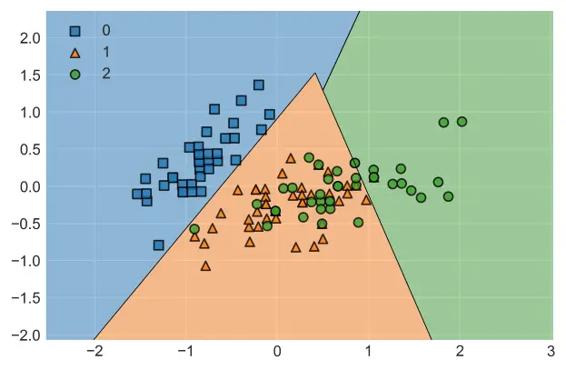
Dimension reduction can be useful because it helps avoid losing valuable training data. However, picking only 2 features can also be useful for visualization purposes sometimes as it makes things more simple to demonstrate. Then, data scientist can return to continuing with full feature set after the visualization and discussions.

b) Dimension Reduction

We will use PCA from sklearn.decomposition module to address this issue of extra dimensions without compromising training data quantity.

from sklearn.decomposition import PCA

SVM = SVC(C=100,gamma=0.0001)
pca = PCA(n_components = 2)
X_train2 = pca.fit_transform(X_train)
SVM.fit(X_train2, y_train)

plot_decision_regions with error “Filler values must be provided when X has more than 2 training features.”

plot_decision_regions(X_train2, y_train, clf=SVM, legend=2, )

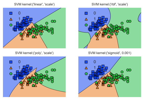
For a multi-plot version of this decision borders chart with demonstrating decision borders with different kernel implementations for SVM you can take a look at the tutorial below:

Tuning Support Vector Machines

c) Confusion Matrix

Another handy visualization tool for classifiers is the confusion matrix.

from sklearn.metrics import plot_confusion_matrix
plot_confusion_matrix(SVM, X_test, y_test, display_labels=data.target_names)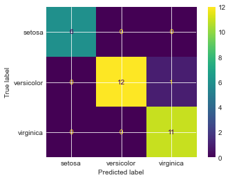

Though a limited dataset in size, we can see that most samples are predicted quite accurately. An exception is 1 versicolor sample which was predicted as virginica which was wrong.

Confusion matrix offers a great opportunity to visualize False True and False False predictions in a very pleasant way and messages is communicated in a very efficient way.

Detective work on the prediction results

6- Support Vector Machine Evaluation

We have a few common tools from sklearn.metrics module that are commonly used in the evaluation of classification models. Below you can see the implementation of the popular scores:

F1 and Jaccard.

We can evaluate the accuracy of decision trees with traditional statistical methods. Below you can see an example of accuracy score applied on our decision tree prediction results on iris dataset.

a) F1 Score

In classification problems we have 4 kind of prediction outcomes in terms of evaluation. These are:

TP: True positive
FP: False positive
TN: True negative
FN: False negative

TN and FN are wrong predictions and they would be unwanted in the outcome as much as possible.

Two metrics commonly used to measure the performance of a machine learning model are: accuracy and precision.

Accuracy is the ratio of True predictions divided by Total predictions. In formulation: (TP+TN) / Total
Precision is the ratio of True positives divided by True and False positives. So, differently, it doesn’t concern itself with predictions of negatives. TP / (TP + FP)
Recall is the ratio of True positives to True positives and False negatives. TP / (TP + FN).

Having laid out those terms, F1 score is the harmonic average of precision and recall. It can be calculated as below using the metrics module of sklearn.

Harmonic mean is a numerical average that can be calculated by dividing the observations amount by reciprocals of each value.

Harmonic mean of 2,5, 6 would be 3 / (1/2 + 1/5 + 1/6) and in F1 score’s case it is:

2 / (1/precision_score + 1/recall_score)

from sklearn.metrics import f1_score
F1_score = f1_score(y_test, yhat, average=None) 
print(F1_score)

[1. 0.92 0.95]

F1 Score is calculated for each predicted class (or target value or label). Above you can see the outcome of our model for labels 0, 1 and 2 representing, setosa, versicolor and virginica kinds of iris plant.

While setosa samples in this model scored a perfect score of 1 for prediction. versicolor and virginica seem to have slightly less desirable prediction outcomes signaling potential room for optimization of our SVM model.

This makes sense since iris dataset has lots of overlap between versicolor and virginica samples’ independent variables (features) while setosa exists in a more easily separable and distant feature space.

b) Jaccard Score

Jaccard score or Jaccard index is another popular metric for classifier evaluation. It can be calculated by dividing the intersect between two classes to the union between two classes.

Union between two classes can be calculated by subtracting intersection from total sample size.

Jaccard index = Intersection / (Total-Intersection) or
Jaccard index = Intersection / Union

In machine learning classifier model evaluation, two samples that are being compared in Jaccard Index are: True labels (often shown as target, y, y_training, y_test) and predicted labels (often shown as yhat, y_pred etc.).

1. with averaging

from sklearn.metrics import jaccard_score
J_score = jaccard_score(y_test, yhat, pos_label=4, average="micro")
print(J_score)

Here we are using micro averaging since there are multiple classes. In this case Jaccard index will be calculated globally meaning total true positives, false negatives and false positives will be counted including all classes.

To see the Jaccard value for each class you can set average parameter to None.

0.9354838709677419

2. without averaging

from sklearn.metrics import jaccard_score
J_score = jaccard_score(y_test, yhat, pos_label=4, average=None)
print(J_score)

Here no averaging is implemented for Jaccard score using None value for average parameter. You can see results are not averaged and Jaccard score returned for each class in the dataset.

[1. 0.88888889 0.92307692]

Summary

In this example component of our Support Vector Machine Tutorial Series we have learned how to implement Support Vector Machine models to solve a classification problem using iris dataset.

As usual, we have also seen some of the intricacies of machine learning and we visualized decision borders of our Support Vector Classifier. Furthermore, we discussed how Tuning can be useful through hyperparameter optimization for improved model outcomes with support vector machines.

Finally, we took a look at a number of evaluation scores such as f1 score and jaccard score to have an idea about how our model is performing.

Thanks for exploring our tutorials about machine learning algorithms.