Logistic Regression Tuning

Optimization of Logistic Regression models can be lots of fun.
Limiting feature amount in the splits
1- penalty
Penalty parameter can be used to specify the norm for regularization in Logistic Regression. In Scikit-Learn’s LogisticRegression implementation, model can take one of the three regularizations: l1, l2 or elasticnet.
parameter value is assigned to l2 by default which means L2 regularization will be applied to the model. Regularization is a method which controls the impact of coefficients and it can result in improved model performance.
parameter value can also be set to None if you’d like to implement no regularization at all. Here is a Python example:
LogR = LogisticRegression(penalty = "elasticnet")
Also please keep in mind that regularization is solver specific. For example:
- l2 works with ‘newton-cg’, ‘sag’, liblinear and ‘lbfgs’ solvers
- ‘elasticnet’ works with ‘saga’ solver
- None works with all solvers except liblinear
LogR = LogisticRegression(C=0.1, penalty='l1', solver='liblinear')
Or for no solvers:
LogR = LogisticRegression(C=0.1, penalty=None, solver='lbfgs')
Here is a summary of regularization and solver compatibility:
l1
- liblinear
- saga
l2
- newton-cg
- lbfgs
- liblinear
- saga
- sag
elasticnet
- saga
None
- newton-cg
- lbfgs
- saga
- sag
Limiting feature amount in the splits
2- C
This is the penalty parameter that controls the extend of regularization. If C is assigned to small values, logistic regression model will have a looser fit on the data. If C is chosen to be too big, this will mean weaker regularization hence potentially increased accuracy.
However, too big C values can cause overfitting problems and this is something that must be kept in mind. C can be seen as the inverse of regularization strength which is denoted by lambda λ in mathematical formulation.
Here is a Python code example to adjust the C parameter:
LogR = LogisticRegression(C = 100)
Limiting feature amount in the splits
3- class_weight
metric parameter is used to define the metric used in distance calculations between samples in DBSCAN algorithm. There are a number of metrics that can be used such as “euclidean” “manhattan” or “minkowski”. If you use “minkowski” metric you can also use p parameter to define the power of minkowski metric.
You can see a Python code for a set of minkowski metric and a p value of 2 below:
LogR = LogisticRegression(C = 100)
Solver Algorithms
4- solver
This parameter defines the solver algorithm used in Logistic Regression. Solver algorithms are used to find solutions to the functions that aim to solve the hypothesis that minimizes the Cost Function (or Loss Function) similar to gradient descent algorithm.
For this reason solver is a dataset dependent choice and lbfgs solver that is assigned by default to the solver parameter usually does a great job for most Logistic Regression applicaitons.
We still have multiple options
- newton-cg: Calculates inverse Hessian explicitly and can be computationally expensive. Useful for small and moderate datasets. newton-cg is what lbfgs is based on.
- lbfgs: Works great with most datasets up to moderate sizes. Current Scikit-Learn default. Instead of explicit full matrix calculations, takes advantage of approximation and remembers recent learning points making computation and space savings. Quasi-Newton solver.
- liblinear: Works great with large linear datasets. Former default solver in Scikit-Learn. No paralellization.
- sag: Only supports L2 regularization. Can be advantageous with large datasets as well as dimensional.
- saga: Sag variant that works with L1, L2 and Elasticnet regularizations. Can be advantageous with big data implementations.
LogR = LogisticRegression(solver = "saga")
Iteration amount for tree structure algorithms in Logistic Regression models
5- max_iter
This parameter is used to out a cap on the maximum iteration of Logistic Regression’s solver algorithm as it attempts to find the global minima of the gradient descent.
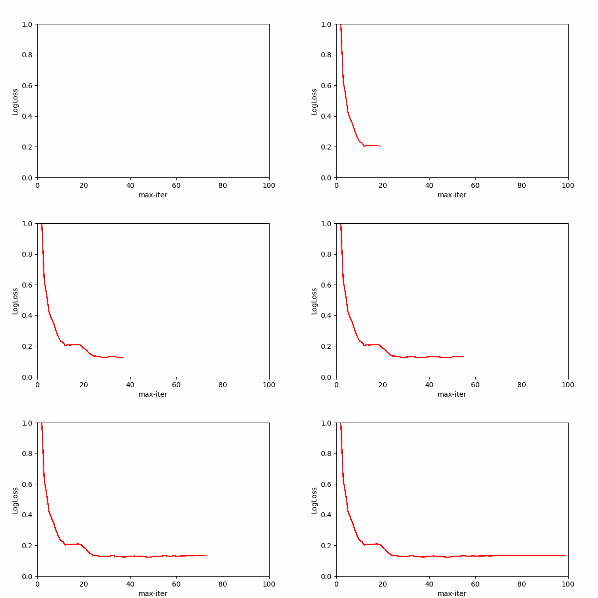
It can be over-blown and you can bring it down using max_iter parameter if you have performance concerns, Here you can see the effects of iteration numbers on the log loss score. Log loss is a classification score that should be minimized for maximum prediction accuracy.

We can see that after each iteration log loss score improves until certain iteration value where log loss improvement stalls. In the animation we can see that most prediction gain is made somewhere around 10th iteration and then some more improvement comes until around 30th iteration. After 70 iteration the line completely stabilizes showing no change on log loss score meaning no change on probability outcomes.
Below you can find the Python code that’s used to create the list of value for the line chart.
lst=[]
from sklearn.metrics import log_loss
for i in range(100):
    LogR = LogisticRegression(n_jobs=-1, max_iter=i)
    LogR.fit(X_train, y_train)

    yhat = LogR.predict(X_test)
    print(LogR.n_iter_)
    print(yhat)
    print(y_test)
    pred = LogR.predict_proba(X_test)
    lst.append(log_loss(y_test, pred))

print(lst)
Furthermore you can use the values in the list to create a matplotlib animation with Python as above using the code below:
from matplotlib.animation import FuncAnimation

fig, axes = plt.subplots(nrows = 1, ncols = 1, figsize = (6,4))
axes.set_ylim(0, 1)
axes.set_xlim(0, 100)

x,y=[], []
plt.xlabel('max-iter', y=-1)
plt.ylabel('LogLoss')

xlst = range(100)
def animate(i):

    y.append(lst[i])
    x.append((xlst[i]))
    plt.plot(x,y,scalex=False,scaley=False, color='red', linewidth=1)

ani = FuncAnimation(fig, animate, interval=100)

#Saving animation as a gif
from matplotlib import animation
f = r"Desktop/animation.gif"
writergif = animation.PillowWriter(fps=30)
ani.save(f, writer=writergif)
Processor paralellization for Logistic Regression
6- n_jobs
n_jobs helps enable a great feature named processor parallelization. It can be used to improve machine learning model performance and Logistic Regression allows paralellization as well. n_jobs is 1 by defult. It can be set to a specific integer (amount of processors desired to work at the same time while the model is in use) or it can be set to -1 to employ all available processors.
LogR = LogisticRegression(n_jobs = 8)
Getting reports from the model in console
6- verbose
Verbose means wordy and it can be used to make the model more explicit while working. If verbose parameter is assigned higher values than its default 0 the model will print increasingly more wordy reports on the console while in use.
Verbosity of Logistic Regression models can be adjusted using the Python code below:
LogR = LogisticRegression(verbose = 5)
Limiting feature amount in the splits
6- warm_start
warm_start can be used to preserve previous learnings of the model. When warm_start is set to True logistic regression model can be retrained without losing the previous learnings. This can be very helpful if your project is based on continuous machine learning or if it is programmed to learn on the go in real time as users make predictions with the model.
Here is a simple demonstration of how you can set warm_start parameter to True using Python:
LogR = LogisticRegression(warm_start = True)
Summary
Logistic Regression is an ancient yet sophisticated machine learning model that is commonly and efficiently used to solve classification problems. It can be very fast, scalable and precise while providing machine learning engineers and data scientists with probability reports. You can read more about pros of Logistic Regression below:
In this Logistic Regression Tutorial, we have explored some of the commonly tuned hyperparameters of Scikit-Learn’s LogisticRegression implementation. We have covered multiple methods to make Logistic Regression faster, more accurate and more reliable through Tuning & Optimization.
Parameters such as verbose, n_jobs, penalty, C, solver, max_iter can offer great opportunities to create a more sophisticated model that with improved machine learning performance.
If you’d like to see more about various algorithm tutorials you can visit: