Logistic Regression Example: Iris

Predicting with built-in Iris dataset

1- Logistic Regression Classifier Model: Training & Prediction

a) Python Libraries for LogisticRegression

We can use LogisticRegression classifier from Scikit-Learn to build a Logistic Regression model for classification. Logistic Regression can only be used for classification problems and it can’t be used to predict continuous values (despite the name “regression“). Thankfully, it does a really good job at what it does: classification.

Let’s import the libraries we’re going to use first.

from sklearn.linear_model import LogisticRegression
from sklearn.model_selection import train_test_split
from sklearn.datasets import load_iris

b) Built-in Iris Dataset

Then we can load iris dataset from Scikit-Learn library’s load_iris module. Let’s explore the data a little bit.

data = load_iris()

print(data.data[:5])
print(data.feature_names)

['sepal length (cm)', 'sepal width (cm)', 'petal length (cm)', 'petal width (cm)']
[[5.1 3.5 1.4 0.2]
[4.9 3. 1.4 0.2]
[4.7 3.2 1.3 0.2]
[4.6 3.1 1.5 0.2]
[5. 3.6 1.4 0.2]]

Class names appear as following:

data = load_iris()

print(data.target[:10])
print(data.target_names)

[0 0 0 0 0 0 0 0 0 0]
['setosa' 'versicolor' 'virginica']

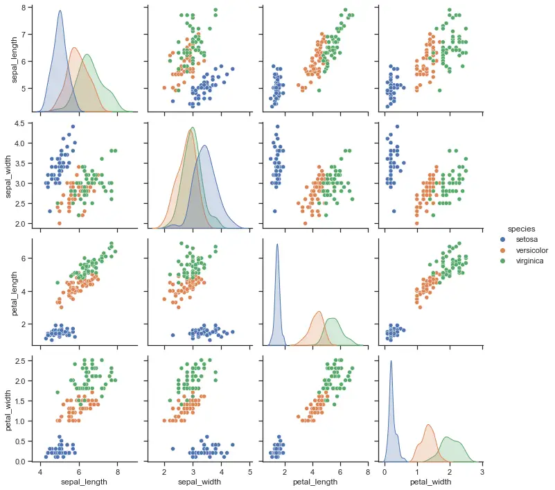
import seaborn as sns
sns.set_theme(style="darkgrid")

df = sns.load_dataset("iris")
sns.pairplot(df, hue="species", palette="icefire")

d) Creating Train Test Split via train_test_split

This part is same for most machine learning tasks. We need to create X_train, X_test, y_train and y_test parts from the dataset.

We can do this task easily by using train_test_split function from sklearn.model_selection module.

X_train, X_test, y_train, y_test = train_test_split(data.data, data.target, test_size=0.2)

Now all the data we need is properly divided between and ready to use for training, predicting and model evaluation.

d) Creating Logistic Regression Classifier

We can create the Random Forest model which we will implement. We can do this by using RandomForestClassifier we’ve already imported.

Let’s create a plain vanilla random forest model with all the default settings:

LogR=LogisticRegression()

You could also create a more custom Logistic Regression model with specific parameters.

You might want to make your model more computationally efficient by activating n_jobs parameter or you can change the penalty criteria and/or penalty strength. More details on Logistic Regression optimization below:

Tuning Random Forest

LogR=LogisticRegression(C=0.02)

e) Training Logistic Regression

We have the model, we have the training data now we can start training the model.

LogR.fit(X_train, y_train)

Logistic Regression is usually a fast classifier model. You can see more about its runtime performance and complexity in the article below:

Logistic Regression Complexity

f) Predicting with Logistic Regression

After training the model it will be ready for use. Here we are making a prediction using the test partition of data without target values.

We can then compare model’s output (yhat) with target values that we already have (y_test) and see how the model is performing.

yhat=LogR.predict(X_test)

print (yhat [0:5])
print (y_test [0:5])

2- ML Expectation Alignment

As the project moves along it’s useful to take a break and consider some aspects of Machine Learning and AI.

Is model suitable for data at hand?
Is training data sufficient for the model?
Do we need probabilistic reports as well as predictions?
Are predictions accurate enough?
What’s the extend of damage when misclassification happens? Harm to health? Injust? Environmental damage? Monetary losses?
Could another model be used for cross-validation?
Is performance good enough?
Will there be a real-time AI deployment?
Are AI ethics considered?
Did we get consent for data collected?
Can ML model be continously trained? (pickling, warm_start)

These are only a fraction of questions that come to mind. Machine learning projects should be assessed from different perspectives by asking questions of similar nature.

Plotting Individual Trees in a Random Forest

3- Logistic Regression Visualization

Logistic Regression can be visualized for different C values as below. This helps make an abstract thought more comprehensible instantly.

a) decision borders based on different C values

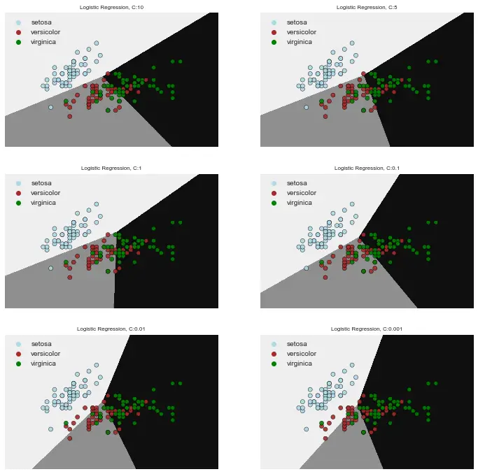
Here is the Python code for multiplot visualization of Logistic Regression decision regions with different C values.

%matplotlib inline
lst = [10, 5, 1, 0.1, 0.01, 0.001, 0.0001]

plt.figure(figsize=(12,12))

for i, j in zip(range(6), lst):
    clf = LogisticRegression(n_jobs=-1, max_iter=19, C=j)
    clf.fit(X, y)
    
    X1min, X1max = X[:, 0].min() - 1, X[:, 0].max() + 1
    X2min, X2max = X[:, 1].min() - 1, X[:, 1].max() + 1
    step = 0.01
    X1, X2 = np.meshgrid(np.arange(X1min, X1max, step), 
                          np.arange(X2min, X2max, step))
    
    Z = clf.predict(np.c_[X1.ravel(), X2.ravel()])
    Z = Z.reshape(X1.shape)
    
    cmap_dots = ['lightblue', 'brown', 'green']
    # plt.figure(dpi=800)
    ax = plt.subplot(3,2,i+1)
    # plt.figure(dpi=800)
    plt.title('Logistic Regression, C:{}'.format(j), size=8); plt.xticks(()); plt.yticks(())
    # plot_decision_regions(X_train2, y_train, clf=LogR, legend=2, colors=colors)
    
    # plt.figure(figsize=(8, 6))
    plt.contourf(X1, X2, Z, cmap="binary")
    
    sns.scatterplot(x=X[:, 0], y=X[:, 1], hue=data.target_names[y],
                    palette=cmap_dots, alpha=0.9, edgecolor="black",)    
    plt.legend(loc='upper left')

b) logloss chart

Another visualization option is to observe the Logloss values of Logistic Regression. Logloss is an important metric that’s used to compare accuracy of classification models. The lower the logloss score the better the model is performing.

lst=[]
from sklearn.metrics import log_loss
for i in range(100):
    LogR = LogisticRegression(n_jobs=-1, max_iter=i)
    LogR.fit(X_train, y_train)
    
    yhat = LogR.predict(X_test)
    print(LogR.n_iter_)
    print(yhat)
    print(y_test)
    pred = LogR.predict_proba(X_test)
    lst.append(log_loss(y_test, pred))

print(lst)

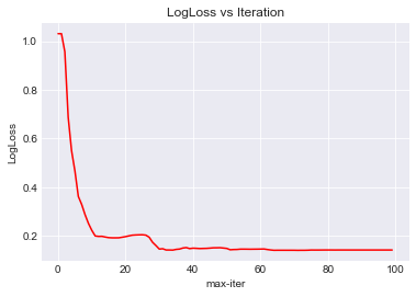
For example in this plot we see that log loss improvement sort of tops around 30 iterations. In a performance conscious model max_iter could be set to 30.

On the other hand even 10 iterations might be enough since that’s where most of the gain is seen. The exact value is dependent on choice and project but this example demonstrates the relationship between logloss value and iterations amount in Logistic Regression models.

Investigating machine learning prediction results

4- Logistic Regression Model Evaluation

Logistic Regression results can be evaluated with the metrics that are used to evaluate most other classification models. Aside of logloss function, we can use conventional metric scores such as F1 and accuracy to see the prediction quality of our model.

from sklearn import metrics
print("LogR Accuracy is: ", metrics.accuracy_score(y_test, yhat))

LogR Accuracy is: 0.9

You may want to tune your logistic regression model after seeing the evaluation metrics and sometimes visualizations:

Tuning Logistic Regression

Some of the criteria regarding tuning based on project specific expectations are:

Accuracy
Performance
Time for training
Simplicity
Computational efficiency
Need for continuing training
Data specific needs (addressing bias, noise, non-linearity) etc.

Summary

In this part of our Logistic Regression Tutorial Series we covered a simple implementation using Random Forest algorithm with built-in Random Forest Classifier model in Scikit-Learn.

We’ve created a Logistic Regression model using LogisticRegression from sklearn.linear_model module. We’ve trained this model to make predictions with it and then we evaluated the prediction results using Scikit-Learn metrics.

Additionally, we have created some plots to visualize the results and working of our Logistic Regression model.

You can also check out our homepage for more Machine Learning Tutorials with Visualizations.